// scenes-v3-overrides.jsx — Institutional variants of scenes 4, 5 and 7.
//
// • S4Aerosols      — drops Popocatépetl (out-of-context for the Valle),
//                     moves the marine-aerosol source higher, pushes the
//                     title below the brand strip.
// • S5Resolution    — embeds the real CAMS/GFS/WRF pixel figure with
//                     proper containment so it can never crop.
// • S6Downscale     — three large source cards: official CAMS icon (SVG),
//                     official WRF logo (PNG) and the SIATA stations map.
//
// Same scene timing / fade behaviour as v2.

// ─── Scene 4 (institutional): aerosol transport — without volcano ────

function S4Aerosols() {
  const { localTime, duration } = useSprite();
  const time = useTime();

  const W = 1280, H = 720;

  // Sources — Valle moved to the far left; burns SE & below the Valle;
  // Caribbean marine aerosol upper-right of Valle (right of burns);
  // Sahara dust stays in its perfect upper-right position.
  const sources = React.useMemo(() => [
    {
      name: 'Polvo del Sahara', tag: 'AOD 1.2', color: C.orange,
      x: 1010, y: 290, spread: 80, weight: 1.0,
    },
    {
      name: 'Quemas · Amazonía', tag: 'BC + OC', color: C.coral,
      x: 600, y: 560, spread: 78, weight: 0.95,
    },
    {
      name: 'Aerosol marino · Caribe', tag: 'sea salt', color: C.cyan,
      x: 720, y: 310, spread: 65, weight: 0.55,
    },
  ], []);

  // Composite trade-wind flow field (unchanged from v2)
  const field = React.useMemo(() => (x, y, t) => {
    const lat = (H / 2 - y) / (H / 2);
    const trade = Math.exp(-lat * lat * 2);
    const vx = -1 * trade - 0.25;
    const vy = lat * 0.25;
    const tt = t * 0.08;
    const swirl = 0.45;
    const cx2 = Math.sin(x * 0.005 + tt) + Math.cos(y * 0.006 - tt * 0.7);
    const cy2 = Math.cos(x * 0.0055 - tt * 0.5) + Math.sin(y * 0.0048 + tt);
    return [vx + cx2 * swirl, vy + cy2 * swirl];
  }, []);

  const totalW = sources.reduce((s, p) => s + p.weight, 0);
  const spawnFn = React.useMemo(() => (t, i) => {
    let pick = (i * 0.6180339 + t * 0.001) % 1;
    pick *= totalW;
    let acc = 0;
    for (const src of sources) {
      acc += src.weight;
      if (pick <= acc) {
        const r = rand(i * 13 + Math.floor(t * 100));
        const ang = r() * Math.PI * 2;
        const rad = Math.sqrt(r()) * src.spread;
        return { x: src.x + Math.cos(ang) * rad, y: src.y + Math.sin(ang) * rad };
      }
    }
    return { x: sources[0].x, y: sources[0].y };
  }, [sources, totalW]);

  const tKick = Easing.easeOutCubic(clamp((localTime - 0.3) / 0.5, 0, 1));
  const tHead = Easing.easeOutCubic(clamp((localTime - 0.7) / 0.7, 0, 1));
  const tMap  = Easing.easeOutCubic(clamp((localTime - 1.0) / 0.8, 0, 1));
  const tPin  = Easing.easeOutCubic(clamp((localTime - 4.0) / 0.6, 0, 1));
  const tFact = Easing.easeOutCubic(clamp((localTime - 6.0) / 0.6, 0, 1));
  const fadeOut = clamp((duration - localTime) / 0.5, 0, 1);

  const valle = { x: 240, y: 360 };

  return (
    <SceneFade>
      <div style={{ opacity: tMap * fadeOut, position: 'absolute', inset: 0 }}>
        <WindyCanvas
          width={W} height={H}
          count={1600}
          field={field}
          spawn={spawnFn}
          palette={[C.orange, C.amber, C.coral, C.cyan, C.rose]}
          fade={0.045}
          speed={1.4}
          life={140}
          lineWidth={1}
          opacity={1}
          background={C.navy}
        />
      </div>

      {/* Source halos */}
      <svg width="1280" height="720" style={{ position: 'absolute', inset: 0, opacity: tMap * fadeOut, pointerEvents: 'none' }}>
        <defs>
          {sources.map((s, i) => (
            <radialGradient key={'rg' + i} id={'srcZone' + i} cx="50%" cy="50%" r="50%">
              <stop offset="0%" stopColor={s.color} stopOpacity="0.22" />
              <stop offset="55%" stopColor={s.color} stopOpacity="0.06" />
              <stop offset="100%" stopColor={s.color} stopOpacity="0" />
            </radialGradient>
          ))}
        </defs>
        {sources.map((s, i) => (
          <ellipse key={'sz' + i} cx={s.x} cy={s.y}
            rx={s.spread * 1.9} ry={s.spread * 1.4}
            fill={'url(#srcZone' + i + ')'} />
        ))}
      </svg>

      {/* Graticule */}
      <svg width="1280" height="720" style={{ position: 'absolute', inset: 0, opacity: tMap * fadeOut, pointerEvents: 'none' }}>
        {[
          { lat: 30, label: '30°N' },
          { lat: 15, label: '15°N' },
          { lat: 0, label: '0°', equator: true },
          { lat: -15, label: '15°S' },
          { lat: -30, label: '30°S' },
        ].map((row, i) => {
          const y = 468 - row.lat * 7.1;
          if (y < 0 || y > 720) return null;
          return (
            <React.Fragment key={'lat' + i}>
              <line x1={0} y1={y} x2={1280} y2={y}
                stroke={C.cyan}
                strokeOpacity={row.equator ? 0.32 : 0.1}
                strokeWidth={row.equator ? 1 : 0.7}
                strokeDasharray={row.equator ? '0' : '3 7'} />
              <text x={20} y={y - 4} fill={C.cyan}
                fillOpacity={row.equator ? 0.6 : 0.32}
                fontFamily={MONO} fontSize={10} letterSpacing="0.12em">{row.label}</text>
            </React.Fragment>
          );
        })}
        {[
          { lon: -90, label: '90°W' },
          { lon: -60, label: '60°W' },
          { lon: -30, label: '30°W' },
          { lon: 0, label: '0°' },
          { lon: 30, label: '30°E' },
        ].map((col, i) => {
          const x = 700 + (col.lon + 75) * 4.13;
          if (x < 0 || x > 1280) return null;
          return (
            <React.Fragment key={'lon' + i}>
              <line x1={x} y1={0} x2={x} y2={720}
                stroke={C.cyan} strokeOpacity={0.08}
                strokeWidth={0.7} strokeDasharray="3 7" />
              <text x={x + 4} y={714} fill={C.cyan}
                fillOpacity={0.32}
                fontFamily={MONO} fontSize={10} letterSpacing="0.12em">{col.label}</text>
            </React.Fragment>
          );
        })}
      </svg>

      {/* Compass — moved right and down a bit so it doesn't fight the brand strip */}
      <div style={{
        position: 'absolute', right: 24, top: 150,
        opacity: tMap * fadeOut, pointerEvents: 'none',
      }}>
        <div style={{
          padding: '10px 14px',
          background: hexWithAlpha(C.ink, 0.6),
          border: '1px solid ' + C.faint,
          borderRadius: 6,
          backdropFilter: 'blur(4px)',
        }}>
          <div style={{
            fontFamily: MONO, fontSize: 9, color: C.gray,
            letterSpacing: '0.18em', textTransform: 'uppercase',
            marginBottom: 6,
          }}>Flujo dominante</div>
          <div style={{ display: 'flex', alignItems: 'center', gap: 10 }}>
            <svg width={36} height={20}>
              <line x1={32} y1={10} x2={6} y2={10} stroke={C.cyan} strokeWidth={1.6} />
              <polygon points="6,10 14,5 14,15" fill={C.cyan} />
            </svg>
            <div style={{
              fontFamily: FONT, fontSize: 12, fontWeight: 600, color: C.cyan,
            }}>E → O</div>
          </div>
          <div style={{
            fontFamily: MONO, fontSize: 9, color: C.gray,
            marginTop: 4, letterSpacing: '0.04em',
          }}>vientos alisios tropicales</div>
        </div>
      </div>

      {/* Header — pushed below the brand strip */}
      <div style={{
        position: 'absolute', left: 24, top: 64, right: 24,
        display: 'flex', justifyContent: 'space-between', alignItems: 'flex-start',
        opacity: fadeOut, pointerEvents: 'none',
      }}>
        <div>
          <div style={{
            fontFamily: MONO, fontSize: 11, fontWeight: 600,
            letterSpacing: '0.26em', textTransform: 'uppercase',
            color: C.cyan,
            opacity: tKick, transform: 'translateY(' + ((1 - tKick) * 8) + 'px)',
          }}>
            Capítulo III · Transporte de aerosoles
          </div>
          <div style={{
            marginTop: 10,
            fontFamily: FONT, fontSize: 28, fontWeight: 700,
            color: C.white, lineHeight: 1.1, letterSpacing: '-0.015em', maxWidth: 540,
            opacity: tHead, transform: 'translateY(' + ((1 - tHead) * 14) + 'px)',
            textShadow: '0 2px 16px rgba(5,10,30,0.9)',
          }}>
            Lo que ven los satélites,<br />
            CAMS lo transporta hora a hora.
          </div>
        </div>
        <div style={{
          textAlign: 'right',
          fontFamily: MONO, fontSize: 11, letterSpacing: '0.16em',
          textTransform: 'uppercase', color: C.gray,
          opacity: tHead, marginTop: 6,
        }}>
          <div style={{ color: C.cyan }}>CAMS Global / aerosol optical depth</div>
          <div style={{ color: C.dim, marginTop: 6 }}>level 550 nm · superficie · UTC {String(Math.floor((time * 6) % 24)).padStart(2, '0')}:00</div>
        </div>
      </div>

      {/* Source pins */}
      {sources.map((s, i) => {
        const ap = Easing.easeOutBack(clamp((localTime - 2.3 - i * 0.2) / 0.5, 0, 1));
        return (
          <div key={i} style={{
            position: 'absolute', left: s.x, top: s.y,
            transform: 'translate(-50%,-50%) scale(' + ap + ')',
            opacity: ap * fadeOut, pointerEvents: 'none',
          }}>
            <div style={{
              position: 'absolute', left: '50%', top: '50%',
              width: 60, height: 60, borderRadius: '50%',
              transform: 'translate(-50%,-50%)',
              background: 'radial-gradient(circle, ' + hexWithAlpha(s.color, 0.35) + ' 0%, ' + hexWithAlpha(s.color, 0) + ' 70%)',
            }} />
            <div style={{
              position: 'absolute', left: '50%', top: '50%',
              transform: 'translate(-50%,-50%)',
              width: 10, height: 10, borderRadius: '50%',
              background: s.color, boxShadow: '0 0 14px ' + s.color,
            }} />
            <div style={{
              position: 'absolute', left: 18, top: -28,
              padding: '6px 10px',
              background: hexWithAlpha(C.ink, 0.78),
              border: '1px solid ' + hexWithAlpha(s.color, 0.4),
              borderRadius: 6, backdropFilter: 'blur(4px)',
              whiteSpace: 'nowrap',
            }}>
              <div style={{ fontFamily: FONT, fontSize: 12, fontWeight: 700, color: s.color }}>{s.name}</div>
              <div style={{ fontFamily: MONO, fontSize: 9.5, color: C.gray, marginTop: 2, letterSpacing: '0.08em' }}>{s.tag}</div>
            </div>
          </div>
        );
      })}

      {/* Valle de Aburrá target */}
      <div style={{
        position: 'absolute', left: valle.x, top: valle.y,
        transform: 'translate(-50%,-50%) scale(' + tPin + ')',
        opacity: tPin * fadeOut, pointerEvents: 'none',
      }}>
        {[0, 1, 2].map(i => {
          const ph = ((time * 0.6 + i / 3) % 1);
          return (
            <div key={i} style={{
              position: 'absolute', left: '50%', top: '50%',
              width: 20 + ph * 80, height: 20 + ph * 80,
              borderRadius: '50%',
              transform: 'translate(-50%,-50%)',
              border: '1.5px solid ' + C.white,
              opacity: (1 - ph) * 0.8,
            }} />
          );
        })}
        <div style={{
          position: 'absolute', left: '50%', top: '50%',
          transform: 'translate(-50%,-50%)',
          width: 16, height: 16, borderRadius: '50%',
          background: C.white,
          boxShadow: '0 0 20px ' + C.white + ', 0 0 40px ' + C.cyan,
        }} />
        <div style={{
          position: 'absolute', left: 24, top: -10,
          padding: '8px 12px',
          background: 'rgba(255,255,255,0.95)',
          borderRadius: 6,
          whiteSpace: 'nowrap',
          boxShadow: '0 4px 24px rgba(0,0,0,0.5)',
        }}>
          <div style={{ fontFamily: FONT, fontSize: 13, fontWeight: 800, color: C.navy }}>Valle de Aburrá</div>
          <div style={{ fontFamily: MONO, fontSize: 9.5, color: C.navy, opacity: 0.65, marginTop: 2, letterSpacing: '0.08em' }}>06°15′N · 75°34′W</div>
        </div>
      </div>

      {/* Bottom fact */}
      <div style={{
        position: 'absolute', left: 24, bottom: 60, right: 24,
        opacity: tFact * fadeOut,
        display: 'flex', justifyContent: 'space-between', alignItems: 'flex-end',
        pointerEvents: 'none',
      }}>
        <div style={{
          maxWidth: 460,
          padding: '14px 18px',
          background: hexWithAlpha(C.ink, 0.78),
          border: '1px solid ' + C.faint,
          borderRadius: 8, backdropFilter: 'blur(6px)',
        }}>
          <div style={{ fontFamily: MONO, fontSize: 10, color: C.cyan, letterSpacing: '0.16em', textTransform: 'uppercase' }}>Por qué importa para el Valle</div>
          <div style={{ fontFamily: FONT, fontSize: 14, color: C.white, lineHeight: 1.5, marginTop: 6 }}>
            Polvo del Sahara, humo de quemas amazónicas y aerosol marino del Caribe
            pueden cruzar el continente en <span style={{ color: C.orange, fontWeight: 700 }}>3 a 5 días</span> y
            modular nuestra calidad del aire local.
          </div>
        </div>
        <div style={{
          fontFamily: MONO, fontSize: 10, color: C.dim,
          letterSpacing: '0.18em', textTransform: 'uppercase',
          textAlign: 'right',
        }}>
          fuente · CAMS global forecast<br />
          <span style={{ color: C.gray }}>aerosol_550nm · superficie</span>
        </div>
      </div>
    </SceneFade>
  );
}

// ─── Scene 5 (institutional): CAMS 40 km pixels over Valle de Aburrá ──

function S5Resolution() {
  const { localTime, duration } = useSprite();
  const time = useTime();

  const tKick = Easing.easeOutCubic(clamp((localTime - 0.2) / 0.5, 0, 1));
  const tHead = Easing.easeOutCubic(clamp((localTime - 0.5) / 0.6, 0, 1));
  const tMap  = Easing.easeOutCubic(clamp((localTime - 1.0) / 0.7, 0, 1));
  const tHL   = Easing.easeOutCubic(clamp((localTime - 2.4) / 0.7, 0, 1));
  const tFact = Easing.easeOutCubic(clamp((localTime - 3.6) / 0.6, 0, 1));
  const fadeOut = clamp((duration - localTime) / 0.45, 0, 1);

  // Smaller image area, contained, so it can't crop. Top a bit lower
  // so it clears the brand strip.
  const mapW = 460, mapH = 520;
  const mapLeft = 760, mapTop = 100;

  const camsPixels = [
    { x: 0.04, y: 0.31 },
    { x: 0.62, y: 0.31 },
    { x: 0.04, y: 0.86 },
    { x: 0.50, y: 0.86 },
    { x: 0.71, y: 0.86 },
    { x: 0.92, y: 0.86 },
  ];

  return (
    <SceneFade>
      <GridBg cell={48} color="rgba(255,255,255,0.018)" />

      <div style={{ position: 'absolute', left: 80, top: 110, width: 440, opacity: fadeOut }}>
        <div style={{
          fontFamily: MONO, fontSize: 11, fontWeight: 600,
          letterSpacing: '0.26em', textTransform: 'uppercase', color: C.cyan,
          opacity: tKick, transform: 'translateY(' + ((1 - tKick) * 8) + 'px)',
        }}>Capítulo IV · El reto de la escala</div>

        <div style={{
          marginTop: 18,
          fontFamily: FONT, fontSize: 38, fontWeight: 700,
          color: C.white, lineHeight: 1.1, letterSpacing: '-0.015em',
          opacity: tHead, transform: 'translateY(' + ((1 - tHead) * 14) + 'px)',
        }}>
          CAMS describe<br />
          el planeta<br />
          en celdas de <span style={{ color: C.orange }}>40&nbsp;km</span>.
        </div>

        <div style={{
          marginTop: 24,
          fontFamily: FONT, fontSize: 15, fontWeight: 400,
          color: C.gray, lineHeight: 1.6,
          opacity: tFact,
          textWrap: 'pretty',
        }}>
          Cada celda promedia <span style={{ color: C.white }}>~1&nbsp;600&nbsp;km²</span> de
          atmósfera. El Valle de Aburrá, con sus <span style={{ color: C.white }}>~60&nbsp;km</span> de
          norte a sur, queda atravesado por sólo
          <span style={{ color: C.cyan, fontWeight: 700 }}> 3 o 4 píxeles</span> CAMS.
        </div>

        <div style={{
          marginTop: 24, padding: '12px 14px',
          background: hexWithAlpha(C.ink, 0.55),
          border: '1px solid ' + C.faint,
          borderRadius: 6,
          opacity: tFact,
        }}>
          <div style={{
            fontFamily: MONO, fontSize: 9.5, color: C.cyan,
            letterSpacing: '0.18em', textTransform: 'uppercase',
            marginBottom: 10,
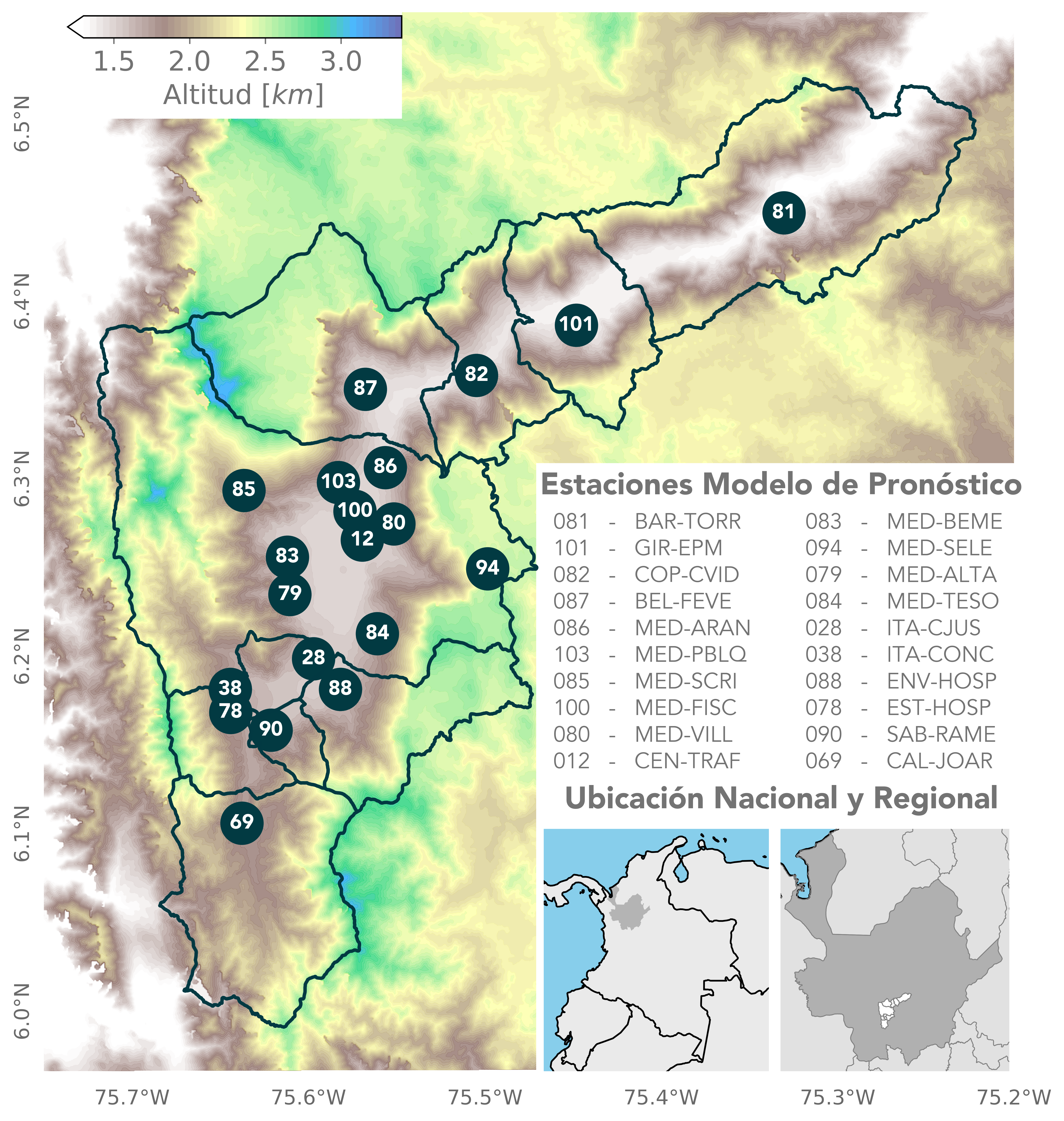
          }}>Resoluciones superpuestas</div>
          {[
            { c: '#A04949', sym: 'square',  l: 'CAMS',       sub: '40 km · global' },
            { c: '#8AA4D4', sym: 'square',  l: 'GFS',        sub: '28 km · global' },
            { c: '#7E7793', sym: 'diamond', l: 'WRF',        sub: '2 km · regional' },
            { c: '#3D1F4A', sym: 'circle',  l: 'Estaciones', sub: '20 puntos · in situ' },
          ].map((row, i) => (
            <div key={i} style={{
              display: 'flex', alignItems: 'center', gap: 10,
              marginBottom: i === 3 ? 0 : 6,
            }}>
              <div style={{
                width: 11, height: 11,
                background: row.c,
                borderRadius: row.sym === 'circle' ? '50%' : 2,
                transform: row.sym === 'diamond' ? 'rotate(45deg)' : 'none',
              }} />
              <div style={{
                fontFamily: FONT, fontSize: 12, fontWeight: 600, color: C.white,
                width: 80,
              }}>{row.l}</div>
              <div style={{
                fontFamily: MONO, fontSize: 9.5, color: C.gray,
                letterSpacing: '0.06em',
              }}>{row.sub}</div>
            </div>
          ))}
        </div>
      </div>

      {/* Right: institutional pixel map — object-contain so it never crops */}
      <div style={{
        position: 'absolute', left: mapLeft, top: mapTop,
        width: mapW, height: mapH,
        opacity: tMap * fadeOut,
      }}>
        <div style={{
          position: 'absolute', inset: 0,
          borderRadius: 6, overflow: 'hidden',
          border: '1px solid ' + hexWithAlpha(C.cyan, 0.25),
          boxShadow: '0 12px 40px rgba(0,0,0,0.5)',
          background: C.ink,
          padding: 4,
        }}>
          <img src="assets/map-data-pixels.png"
            alt="CAMS, GFS, WRF pixels y estaciones SIATA sobre el Valle de Aburrá"
            style={{
              width: '100%', height: '100%', objectFit: 'contain',
              display: 'block',
            }} />

          {/* Highlight pulses on the red CAMS pixels */}
          <svg width="100%" height="100%" style={{
            position: 'absolute', inset: 0, pointerEvents: 'none',
            opacity: tHL,
          }} viewBox="0 0 100 100" preserveAspectRatio="none">
            {camsPixels.map((p, i) => {
              const ph = ((time * 0.55 + i * 0.18) % 1);
              const r = 2 + ph * 5;
              return (
                <circle key={i}
                  cx={p.x * 100} cy={p.y * 100}
                  r={r}
                  fill="none" stroke={C.cyan}
                  strokeWidth={0.4}
                  strokeOpacity={(1 - ph) * 0.8} />
              );
            })}
          </svg>
        </div>

        <div style={{
          position: 'absolute', left: 0, bottom: -28, right: 0,
          fontFamily: MONO, fontSize: 10, color: C.gray,
          letterSpacing: '0.04em', textAlign: 'center',
          opacity: tFact,
        }}>
          <span style={{ color: C.white, fontWeight: 600 }}>Fig. 1</span>
          &nbsp;· Píxeles de modelos meteorológicos sobre el Valle de Aburrá
        </div>
      </div>
    </SceneFade>
  );
}

// ─── Scene 7 (institutional): Ensamble local — three big source cards ──

function S6Downscale() {
  const { localTime, duration } = useSprite();
  const time = useTime();

  const tKick = Easing.easeOutCubic(clamp((localTime - 0.2) / 0.5, 0, 1));
  const tHead = Easing.easeOutCubic(clamp((localTime - 0.6) / 0.6, 0, 1));
  const tCams = Easing.easeOutCubic(clamp((localTime - 1.2) / 0.6, 0, 1));
  const tWrf  = Easing.easeOutCubic(clamp((localTime - 1.8) / 0.6, 0, 1));
  const tStn  = Easing.easeOutCubic(clamp((localTime - 2.4) / 0.6, 0, 1));
  const tArr  = Easing.easeOutCubic(clamp((localTime - 3.4) / 0.7, 0, 1));
  const tOut  = Easing.easeOutCubic(clamp((localTime - 4.4) / 0.7, 0, 1));
  const tCap  = Easing.easeOutCubic(clamp((localTime - 5.5) / 0.6, 0, 1));
  const fadeOut = clamp((duration - localTime) / 0.45, 0, 1);

  // Cards stack: each is "highlighted" briefly as its arrow fires.
  const cardW = 320, cardH = 150, cardX = 56;
  const inputs = [
    {
      key: 'cams',
      label: 'CAMS · 40 km',
      sub: 'background químico',
      color: C.orange,
      t: tCams,
      highlight: 1.2,
      y: 170,
      kind: 'cams-icon',
    },
    {
      key: 'wrf',
      label: 'WRF · 2 km',
      sub: 'meteorología regional',
      color: C.cyan,
      t: tWrf,
      highlight: 1.8,
      y: 340,
      kind: 'wrf-logo',
    },
    {
      key: 'stn',
      label: '20 estaciones SIATA',
      sub: 'PM2.5 in situ',
      color: C.amber,
      t: tStn,
      highlight: 2.4,
      y: 510,
      kind: 'stations-map',
    },
  ];

  // CAMS icon comes from the official Copernicus Atmosphere SVG —
  // see assets/cams-icon.svg. We load it via <img> so its original
  // teal (#55bfd0) is preserved untouched.

  return (
    <SceneFade>
      <GridBg cell={48} color="rgba(255,255,255,0.018)" />

      {/* Header */}
      <div style={{
        position: 'absolute', left: '50%', top: 64,
        transform: 'translateX(-50%)', textAlign: 'center',
        opacity: fadeOut,
      }}>
        <div style={{
          fontFamily: MONO, fontSize: 11, fontWeight: 600,
          letterSpacing: '0.26em', textTransform: 'uppercase', color: C.cyan,
          opacity: tKick, transform: 'translateY(' + ((1 - tKick) * 6) + 'px)',
        }}>Capítulo VI · Ensamble local</div>
        <div style={{
          marginTop: 12,
          fontFamily: FONT, fontSize: 30, fontWeight: 700,
          color: C.white, letterSpacing: '-0.015em',
          opacity: tHead, transform: 'translateY(' + ((1 - tHead) * 12) + 'px)',
        }}>
          Del modelo global a <span style={{ color: C.cyan }}>cada estación</span> SIATA
        </div>
      </div>

      {/* Input cards — large, with real institutional refs */}
      {inputs.map((inp, i) => {
        const pulse = Math.max(0, 1 - Math.abs(localTime - inp.highlight) * 1.4);
        const lift = pulse * 6;
        return (
          <div key={inp.key} style={{
            position: 'absolute', left: cardX, top: inp.y,
            width: cardW, height: cardH,
            opacity: inp.t * fadeOut,
            transform: 'translate(' + ((1 - inp.t) * -20) + 'px, ' + (-lift) + 'px)',
          }}>
            {/* Card */}
            <div style={{
              position: 'absolute', inset: 0,
              border: '1px solid ' + hexWithAlpha(inp.color, 0.35 + pulse * 0.4),
              borderRadius: 8,
              background: hexWithAlpha(C.ink, 0.7),
              boxShadow: pulse > 0.05
                ? '0 0 28px ' + hexWithAlpha(inp.color, pulse * 0.45)
                : 'none',
              transition: 'box-shadow 0.2s',
            }} />
            {/* Big institutional thumbnail (left half of card) */}
            <div style={{
              position: 'absolute', left: 14, top: 14,
              width: cardH - 28, height: cardH - 28,
              borderRadius: 6, overflow: 'hidden',
              background: inp.kind === 'cams-icon'
                ? hexWithAlpha(C.white, 0.04)
                : C.white,
              display: 'flex', alignItems: 'center', justifyContent: 'center',
            }}>
              {inp.kind === 'cams-icon' && (
                <img src="assets/cams-icon.svg" alt="Copernicus Atmosphere · CAMS"
                  style={{ width: '78%', height: '78%', objectFit: 'contain' }} />
              )}
              {inp.kind === 'wrf-logo' && (
                <img src="assets/wrf-logo.png" alt="WRF logo"
                  style={{ width: '92%', height: '92%', objectFit: 'contain' }} />
              )}
              {inp.kind === 'stations-map' && (
                <img src="assets/ForW_PM25.png" alt="Mapa de estaciones SIATA"
                  style={{
                    width: '100%', height: '100%', objectFit: 'cover',
                    objectPosition: '20% 50%',
                  }} />
              )}
            </div>
            {/* Label on right */}
            <div style={{
              position: 'absolute', left: cardH + 4, top: 22, right: 14,
            }}>
              <div style={{ fontFamily: FONT, fontSize: 16, fontWeight: 700, color: inp.color, lineHeight: 1.2 }}>{inp.label}</div>
              <div style={{ fontFamily: MONO, fontSize: 10, color: C.gray, letterSpacing: '0.08em', marginTop: 6 }}>{inp.sub}</div>
              {inp.key === 'cams' && (
                <div style={{ fontFamily: FONT, fontSize: 11, color: C.dim, marginTop: 12, lineHeight: 1.45 }}>
                  Copernicus · ECMWF<br />química global, hora a hora
                </div>
              )}
              {inp.key === 'wrf' && (
                <div style={{ fontFamily: FONT, fontSize: 11, color: C.dim, marginTop: 12, lineHeight: 1.45 }}>
                  NCAR · UCAR<br />viento, T, humedad, capa límite
                </div>
              )}
              {inp.key === 'stn' && (
                <div style={{ fontFamily: FONT, fontSize: 11, color: C.dim, marginTop: 12, lineHeight: 1.45 }}>
                  Red Calidad del Aire AMVA<br />muestreo horario, 24/7
                </div>
              )}
            </div>
          </div>
        );
      })}

      {/* Arrows + ML node */}
      <svg width="1280" height="720" style={{ position: 'absolute', inset: 0, opacity: tArr * fadeOut }}>
        {inputs.map((inp) => {
          const sy = inp.y + cardH / 2;
          return (
            <line key={inp.key} x1={cardX + cardW + 6} y1={sy} x2={600} y2={400}
              stroke={inp.color} strokeWidth={1.4} strokeOpacity={0.55}
              strokeDasharray="4 4" />
          );
        })}
        <line x1={740} y1={400} x2={900} y2={400}
          stroke={C.green} strokeWidth={1.8} strokeOpacity={0.7} />
        <polygon points="900,395 910,400 900,405" fill={C.green} fillOpacity={0.85} />
        {inputs.map((inp, i) => {
          const ph = ((time * 0.5 + i * 0.33) % 1);
          const x = (cardX + cardW + 6) + (600 - (cardX + cardW + 6)) * ph;
          const y = (inp.y + cardH / 2) + (400 - (inp.y + cardH / 2)) * ph;
          return <circle key={'pp' + i} cx={x} cy={y} r={3} fill={inp.color} opacity={(1 - ph) * 0.95} />;
        })}
      </svg>

      {/* ML node */}
      <div style={{
        position: 'absolute', left: 670, top: 400,
        transform: 'translate(-50%,-50%) scale(' + (Easing.easeOutBack(clamp((localTime - 3.2) / 0.6, 0, 1))) + ')',
        opacity: tArr * fadeOut,
      }}>
        <div style={{
          width: 130, height: 130, borderRadius: '50%',
          background: C.coral,
          display: 'flex', flexDirection: 'column',
          alignItems: 'center', justifyContent: 'center',
          boxShadow: '0 0 36px ' + hexWithAlpha(C.coral, 0.4) + ', 0 0 70px ' + hexWithAlpha(C.coral, 0.18),
        }}>
          <div style={{
            fontFamily: FONT, fontSize: 12, fontWeight: 800,
            color: C.white, letterSpacing: '0.05em',
            textTransform: 'uppercase', textAlign: 'center',
          }}>Machine<br />Learning</div>
          <div style={{
            fontFamily: MONO, fontSize: 9, color: 'rgba(255,255,255,0.7)',
            marginTop: 6, letterSpacing: '0.12em',
          }}>ensamble</div>
        </div>
      </div>

      {/* Output heatmap */}
      <div style={{
        position: 'absolute', left: 900, top: 220,
        opacity: tOut * fadeOut,
        transform: 'translateX(' + ((1 - tOut) * 20) + 'px)',
      }}>
        <div style={{
          fontFamily: MONO, fontSize: 10, color: C.cyan,
          letterSpacing: '0.2em', textTransform: 'uppercase',
          marginBottom: 12,
        }}>Pronóstico · 20 estaciones × 72 h</div>

        <div style={{
          position: 'relative',
          padding: 12,
          border: '1px solid ' + hexWithAlpha(C.green, 0.4),
          borderRadius: 8,
          background: hexWithAlpha(C.ink, 0.55),
        }}>
          <div style={{
            display: 'flex', justifyContent: 'space-between',
            marginBottom: 6, paddingLeft: 28,
            fontFamily: MONO, fontSize: 8.5, color: C.dim, letterSpacing: '0.08em',
          }}>
            <span>T+0</span><span>+24h</span><span>+48h</span><span>+72h</span>
          </div>

          {Array.from({ length: 20 }, (_, row) => (
            <div key={row} style={{
              display: 'flex', alignItems: 'center', gap: 4,
              marginBottom: 1.5,
            }}>
              <div style={{
                width: 22,
                fontFamily: MONO, fontSize: 8, color: C.gray,
                letterSpacing: '0.06em', textAlign: 'right',
              }}>E{String(row + 1).padStart(2, '0')}</div>
              <div style={{
                display: 'grid',
                gridTemplateColumns: 'repeat(24, 1fr)',
                gap: 1,
                width: 192,
              }}>
                {Array.from({ length: 24 }, (_, col) => {
                  const stationLevel = 0.4 + (Math.sin(row * 1.3) + 1) / 2 * 0.5;
                  const phase = col / 24 * Math.PI * 6 + row * 0.18;
                  const diurnal = (Math.sin(phase - Math.PI / 2) + 1) / 2;
                  const drift = (Math.sin(col * 0.18 + row * 0.07) + 1) / 2 * 0.3;
                  const v = stationLevel * (0.4 + diurnal * 0.5) + drift;
                  const color = v > 0.75 ? C.coral
                             : v > 0.55 ? C.orange
                             : v > 0.35 ? C.amber
                             : C.green;
                  const ap = Easing.easeOutCubic(clamp((localTime - 4.4 - (row + col) * 0.02) / 0.4, 0, 1));
                  return (
                    <div key={col} style={{
                      height: 5,
                      background: hexWithAlpha(color, 0.35 + v * 0.55),
                      opacity: ap,
                    }} />
                  );
                })}
              </div>
            </div>
          ))}

          <div style={{
            display: 'flex', alignItems: 'center', gap: 8,
            marginTop: 12, paddingLeft: 28,
          }}>
            <div style={{
              flex: 1, height: 6, borderRadius: 3,
              background: 'linear-gradient(90deg,' + C.green + ',' + C.amber + ',' + C.orange + ',' + C.coral + ')',
            }} />
          </div>
          <div style={{
            display: 'flex', justifyContent: 'space-between',
            marginTop: 4, paddingLeft: 28,
            fontFamily: MONO, fontSize: 8.5, color: C.dim, letterSpacing: '0.08em',
          }}>
            <span>0</span><span>µg/m³</span><span>50+</span>
          </div>
        </div>
      </div>

      {/* Bottom caption */}
      <div style={{
        position: 'absolute', left: 56, bottom: 60, right: 56,
        opacity: tCap * fadeOut, textAlign: 'center',
      }}>
        <div style={{
          fontFamily: FONT, fontSize: 14, color: C.gray, lineHeight: 1.5,
          maxWidth: 880, margin: '0 auto', textWrap: 'pretty',
        }}>
          Modelos de <span style={{ color: C.white }}>machine learning</span> aprenden a corregir el sesgo de CAMS
          <span style={{ color: C.white }}> en la coordenada exacta</span> de cada estación,
          usando WRF como contexto meteorológico y los <span style={{ color: C.white }}>datos históricos</span> de
          PM<span style={{ fontSize: 11 }}>2.5</span> como anclaje real.
        </div>
      </div>
    </SceneFade>
  );
}

// ─── Scene 6 (institutional): ¿Qué es WRF? — equations + 2 km ─────────

function S6WRF() {
  const { localTime, duration } = useSprite();
  const time = useTime();

  const tKick  = Easing.easeOutCubic(clamp((localTime - 0.2) / 0.5, 0, 1));
  const tHead  = Easing.easeOutCubic(clamp((localTime - 0.6) / 0.6, 0, 1));
  const tBody  = Easing.easeOutCubic(clamp((localTime - 1.1) / 0.7, 0, 1));
  const tEq    = Easing.easeOutCubic(clamp((localTime - 1.8) / 0.6, 0, 1));
  const tD1    = Easing.easeOutCubic(clamp((localTime - 2.2) / 0.5, 0, 1));
  const tD2    = Easing.easeOutCubic(clamp((localTime - 2.7) / 0.5, 0, 1));
  const tD3    = Easing.easeOutCubic(clamp((localTime - 3.2) / 0.5, 0, 1));
  const tWinds = Easing.easeOutCubic(clamp((localTime - 3.9) / 0.6, 0, 1));
  const tStats = Easing.easeOutCubic(clamp((localTime - 4.7) / 0.6, 0, 1));
  const fadeOut = clamp((duration - localTime) / 0.45, 0, 1);

  const cx = 920, cy = 400;
  const d1 = { w: 320, h: 360, color: C.purple, label: 'D01 · 18 km', sub: 'NW de Sudamérica' };
  const d2 = { w: 200, h: 230, color: C.cyan,   label: 'D02 · 9 km',  sub: 'Antioquia' };
  const d3 = { w: 110, h: 140, color: C.amber,  label: 'D03 · 2 km',  sub: 'Valle de Aburrá' };

  return (
    <SceneFade>
      <GridBg cell={48} color="rgba(255,255,255,0.018)" />

      {/* Left text column */}
      <div style={{
        position: 'absolute', left: 80, top: 110, width: 460,
        opacity: fadeOut,
      }}>
        <div style={{
          fontFamily: MONO, fontSize: 11, fontWeight: 600,
          letterSpacing: '0.26em', textTransform: 'uppercase', color: C.cyan,
          opacity: tKick, transform: 'translateY(' + ((1 - tKick) * 8) + 'px)',
        }}>
          Capítulo V · ¿Qué es WRF?
        </div>

        <div style={{
          marginTop: 16,
          fontFamily: FONT, fontSize: 38, fontWeight: 700,
          color: C.white, lineHeight: 1.1, letterSpacing: '-0.015em',
          opacity: tHead, transform: 'translateY(' + ((1 - tHead) * 14) + 'px)',
        }}>
          La <span style={{ color: C.amber }}>meteorología</span><br />
          del Valle,<br />
          hora a hora.
        </div>

        <div style={{
          marginTop: 22,
          fontFamily: FONT, fontSize: 15, fontWeight: 400,
          color: C.gray, lineHeight: 1.6, maxWidth: 420,
          opacity: tBody, transform: 'translateY(' + ((1 - tBody) * 12) + 'px)',
          textWrap: 'pretty',
        }}>
          <span style={{ color: C.white }}>WRF</span> (Weather Research &amp; Forecasting,
          NCAR&nbsp;/&nbsp;UCAR) resuelve, en cada celda del modelo,
          <span style={{ color: C.white }}> las ecuaciones del movimiento del aire</span>:
          conservación de masa, energía, momento y humedad.
        </div>

        {/* Equation block */}
        <div style={{
          marginTop: 18,
          padding: '12px 16px',
          background: hexWithAlpha(C.ink, 0.6),
          border: '1px solid ' + hexWithAlpha(C.amber, 0.3),
          borderRadius: 6,
          opacity: tEq, transform: 'translateY(' + ((1 - tEq) * 10) + 'px)',
        }}>
          <div style={{
            fontFamily: MONO, fontSize: 9.5, color: C.amber,
            letterSpacing: '0.18em', textTransform: 'uppercase',
            marginBottom: 8,
          }}>Ecuaciones primitivas</div>
          <div style={{
            fontFamily: MONO, fontSize: 13, color: C.white,
            lineHeight: 1.6, letterSpacing: '0.02em',
          }}>
            <div>∂<span style={{ color: C.cyan }}>u</span>/∂t = − v·∇u − fk×v − (1/ρ)∇p + F</div>
            <div>∂<span style={{ color: C.cyan }}>θ</span>/∂t = − v·∇θ + Q/Π</div>
            <div>∂<span style={{ color: C.cyan }}>q</span>/∂t = − v·∇q + S<sub>q</sub></div>
          </div>
          <div style={{
            marginTop: 8,
            fontFamily: MONO, fontSize: 9.5, color: C.gray,
            letterSpacing: '0.04em', lineHeight: 1.4,
          }}>
            viento · temperatura potencial · humedad
          </div>
        </div>

        <div style={{
          marginTop: 18,
          fontFamily: FONT, fontSize: 14, fontWeight: 400,
          color: C.gray, lineHeight: 1.55, maxWidth: 420,
          opacity: tBody,
          textWrap: 'pretty',
        }}>
          SIATA opera WRF con <span style={{ color: C.white }}>tres dominios anidados</span> que
          bajan de 18 km a <span style={{ color: C.amber }}>2 km</span> sobre el Valle,
          capturando el efecto de las montañas que CAMS no puede ver.
        </div>

        {/* Stats pills */}
        <div style={{
          marginTop: 24, display: 'flex', gap: 10, flexWrap: 'wrap',
          opacity: tStats,
        }}>
          {[
            { v: '2 km', l: 'dominio interno' },
            { v: '16', l: 'variables' },
            { v: 'horaria', l: 'salida' },
          ].map((s, i) => (
            <div key={i} style={{
              padding: '8px 12px',
              border: '1px solid ' + C.faint,
              borderRadius: 6, background: 'rgba(255,255,255,0.025)',
            }}>
              <div style={{ fontFamily: FONT, fontSize: 16, fontWeight: 700, color: C.white }}>{s.v}</div>
              <div style={{ fontFamily: MONO, fontSize: 9.5, color: C.gray, letterSpacing: '0.1em', textTransform: 'uppercase', marginTop: 2 }}>{s.l}</div>
            </div>
          ))}
        </div>
      </div>

      {/* Right diagram: nested WRF domains — D01 18 km, D02 9 km, D03 3 km */}
      <div style={{ position: 'absolute', left: cx, top: cy, opacity: fadeOut }}>
        {/* D01 */}
        <div style={{
          position: 'absolute', left: -d1.w / 2, top: -d1.h / 2,
          width: d1.w, height: d1.h,
          border: '1.5px solid ' + hexWithAlpha(d1.color, 0.5),
          background: hexWithAlpha(d1.color, 0.04),
          borderRadius: 4,
          opacity: tD1, transform: 'scale(' + (0.92 + 0.08 * tD1) + ')',
        }}>
          <svg width={d1.w} height={d1.h} style={{ position: 'absolute', inset: 0, opacity: 0.5 }}>
            {Array.from({ length: 8 }, (_, i) => (
              <line key={'h' + i} x1={0} y1={(d1.h / 8) * i} x2={d1.w} y2={(d1.h / 8) * i}
                stroke={d1.color} strokeOpacity={0.18} strokeWidth={0.6} />
            ))}
            {Array.from({ length: 7 }, (_, i) => (
              <line key={'v' + i} x1={(d1.w / 7) * i} y1={0} x2={(d1.w / 7) * i} y2={d1.h}
                stroke={d1.color} strokeOpacity={0.18} strokeWidth={0.6} />
            ))}
          </svg>
          <div style={{
            position: 'absolute', left: 8, top: 6,
            fontFamily: MONO, fontSize: 10, fontWeight: 700,
            color: d1.color, letterSpacing: '0.16em',
          }}>{d1.label}</div>
          <div style={{
            position: 'absolute', left: 8, top: 22,
            fontFamily: MONO, fontSize: 9, color: C.gray,
            letterSpacing: '0.08em',
          }}>{d1.sub}</div>
        </div>

        {/* D02 */}
        <div style={{
          position: 'absolute', left: -d2.w / 2 + 10, top: -d2.h / 2 - 10,
          width: d2.w, height: d2.h,
          border: '1.5px solid ' + hexWithAlpha(d2.color, 0.6),
          background: hexWithAlpha(d2.color, 0.06),
          borderRadius: 4,
          opacity: tD2, transform: 'scale(' + (0.9 + 0.1 * tD2) + ')',
        }}>
          <svg width={d2.w} height={d2.h} style={{ position: 'absolute', inset: 0, opacity: 0.6 }}>
            {Array.from({ length: 12 }, (_, i) => (
              <line key={'h' + i} x1={0} y1={(d2.h / 12) * i} x2={d2.w} y2={(d2.h / 12) * i}
                stroke={d2.color} strokeOpacity={0.2} strokeWidth={0.5} />
            ))}
            {Array.from({ length: 10 }, (_, i) => (
              <line key={'v' + i} x1={(d2.w / 10) * i} y1={0} x2={(d2.w / 10) * i} y2={d2.h}
                stroke={d2.color} strokeOpacity={0.2} strokeWidth={0.5} />
            ))}
          </svg>
          <div style={{
            position: 'absolute', left: 8, top: 6,
            fontFamily: MONO, fontSize: 10, fontWeight: 700,
            color: d2.color, letterSpacing: '0.16em',
          }}>{d2.label}</div>
          <div style={{
            position: 'absolute', left: 8, top: 22,
            fontFamily: MONO, fontSize: 9, color: C.gray,
            letterSpacing: '0.08em',
          }}>{d2.sub}</div>
        </div>

        {/* D03 — Valle de Aburrá at 2 km */}
        <div style={{
          position: 'absolute', left: -d3.w / 2 + 22, top: -d3.h / 2 - 4,
          width: d3.w, height: d3.h,
          border: '2px solid ' + hexWithAlpha(d3.color, 0.85),
          background: hexWithAlpha(d3.color, 0.08),
          borderRadius: 4,
          opacity: tD3,
          transform: 'scale(' + (0.85 + 0.15 * tD3) + ')',
          boxShadow: '0 0 20px ' + hexWithAlpha(d3.color, 0.35),
        }}>
          <svg width={d3.w} height={d3.h} style={{ position: 'absolute', inset: 0 }}>
            {Array.from({ length: 14 }, (_, i) => (
              <line key={'h' + i} x1={0} y1={(d3.h / 14) * i} x2={d3.w} y2={(d3.h / 14) * i}
                stroke={d3.color} strokeOpacity={0.18} strokeWidth={0.4} />
            ))}
            {Array.from({ length: 11 }, (_, i) => (
              <line key={'v' + i} x1={(d3.w / 11) * i} y1={0} x2={(d3.w / 11) * i} y2={d3.h}
                stroke={d3.color} strokeOpacity={0.18} strokeWidth={0.4} />
            ))}
            <path d={'M ' + (d3.w / 2) + ' 12 C ' + (d3.w / 2 + 12) + ' 36, ' + (d3.w / 2 + 16) + ' 70, ' + (d3.w / 2 + 12) + ' 100 C ' + (d3.w / 2 + 6) + ' 120, ' + (d3.w / 2) + ' ' + (d3.h - 12) + ', ' + (d3.w / 2) + ' ' + (d3.h - 12) + ' C ' + (d3.w / 2 - 6) + ' 120, ' + (d3.w / 2 - 16) + ' 70, ' + (d3.w / 2 - 12) + ' 36 C ' + (d3.w / 2 - 8) + ' 24, ' + (d3.w / 2) + ' 12, ' + (d3.w / 2) + ' 12 Z'}
              fill={hexWithAlpha(C.white, 0.08)} stroke={C.white} strokeOpacity={0.4} strokeWidth={0.8} />
            {tWinds > 0 && (() => {
              const arrows = [];
              for (let i = 0; i < 5; i++) {
                for (let j = 0; j < 7; j++) {
                  const ax = 10 + (d3.w - 20) * (i + 0.5) / 5;
                  const ay = 12 + (d3.h - 24) * (j + 0.5) / 7;
                  const phase = time * 0.6 + j * 0.3;
                  const ang = -Math.PI / 2 + Math.sin(phase) * 0.5;
                  const len = 6 + 3 * Math.sin(phase + i);
                  const ex = ax + Math.cos(ang) * len;
                  const ey = ay + Math.sin(ang) * len;
                  const opa = tWinds * (0.45 + Math.sin(phase + i * 0.7) * 0.25);
                  arrows.push(
                    <g key={'a' + i + '_' + j}>
                      <line x1={ax} y1={ay} x2={ex} y2={ey}
                        stroke={C.white} strokeOpacity={opa} strokeWidth={0.9} />
                      <circle cx={ex} cy={ey} r={1.2} fill={C.white} opacity={opa} />
                    </g>
                  );
                }
              }
              return arrows;
            })()}
          </svg>
          <div style={{
            position: 'absolute', left: '50%', bottom: -22,
            transform: 'translateX(-50%)',
            fontFamily: MONO, fontSize: 10, fontWeight: 700,
            color: d3.color, letterSpacing: '0.16em',
            whiteSpace: 'nowrap',
          }}>{d3.label}</div>
        </div>
      </div>
    </SceneFade>
  );
}

// ─── Scene 9 (institutional): Outro — final phrase with WRF nod ───────

function S8Outro() {
  const { localTime, duration } = useSprite();
  const time = useTime();

  const field = React.useMemo(() =>
    directionalField(Math.PI * 0.98, 0.0035, 0.15, 0.55, 0.4), []);

  const tKick = Easing.easeOutCubic(clamp((localTime - 0.3) / 0.5, 0, 1));
  const tHead = Easing.easeOutCubic(clamp((localTime - 0.7) / 0.7, 0, 1));
  const tFoot = Easing.easeOutCubic(clamp((localTime - 3.0) / 0.5, 0, 1));
  const fadeOut = clamp((duration - localTime) / 0.6, 0, 1);

  const stats = [
    { v: '4', l: 'fuentes integradas', c: C.cyan, d: 0 },
    { v: '20', l: 'estaciones SIATA', c: C.amber, d: 0.15 },
    { v: '72 h', l: 'horizonte de pronóstico', c: C.orange, d: 0.3, nowrap: true },
    { v: '>80%', l: 'acierto categoría ICA', c: C.green, d: 0.45 },
  ];

  return (
    <SceneFade>
      <WindyCanvas
        width={1280} height={720}
        count={750}
        field={field}
        palette={[C.cyan, C.sky, C.orange, C.amber, C.green]}
        fade={0.08}
        speed={0.6}
        life={140}
        lineWidth={1}
        opacity={0.55}
        background={C.navy}
      />

      <div style={{
        position: 'absolute', inset: 0,
        background: 'radial-gradient(ellipse at 50% 50%, rgba(10,37,64,0) 25%, rgba(10,37,64,0.9) 95%)',
        pointerEvents: 'none',
      }} />

      <div style={{
        position: 'absolute', left: '50%', top: 140,
        transform: 'translateX(-50%)', textAlign: 'center',
        opacity: fadeOut,
      }}>
        <div style={{
          fontFamily: MONO, fontSize: 12, fontWeight: 600,
          letterSpacing: '0.32em', textTransform: 'uppercase', color: C.cyan,
          opacity: tKick, transform: 'translateY(' + ((1 - tKick) * 8) + 'px)',
        }}>El círculo se cierra</div>

        <div style={{
          marginTop: 22,
          fontFamily: FONT, fontSize: 44, fontWeight: 800,
          color: C.white, lineHeight: 1.18, letterSpacing: '-0.02em',
          opacity: tHead, transform: 'translateY(' + ((1 - tHead) * 16) + 'px)',
          maxWidth: 980, margin: '0 auto',
          textShadow: '0 4px 24px rgba(10,37,64,0.8)',
        }}>
          CAMS observa el planeta.<br />
          <span style={{
            background: 'linear-gradient(90deg,' + C.cyan + ',' + C.green + ')',
            WebkitBackgroundClip: 'text', WebkitTextFillColor: 'transparent',
            backgroundClip: 'text', color: 'transparent',
          }}>SIATA lo aterriza al Valle con ciencia y modelos propios.</span>
        </div>
      </div>

      {/* Stats grid */}
      <div style={{
        position: 'absolute', left: '50%', top: 380,
        transform: 'translateX(-50%)',
        display: 'flex', gap: 56, alignItems: 'flex-start',
        opacity: fadeOut,
      }}>
        {stats.map((s, i) => {
          const ap = Easing.easeOutBack(clamp((localTime - 1.5 - s.d) / 0.6, 0, 1));
          return (
            <div key={i} style={{
              textAlign: 'center',
              opacity: ap,
              transform: 'translateY(' + ((1 - ap) * 18) + 'px)',
            }}>
              <div style={{
                fontFamily: FONT, fontSize: 54, fontWeight: 800,
                color: s.c, lineHeight: 1,
                whiteSpace: 'nowrap',
                textShadow: '0 0 24px ' + hexWithAlpha(s.c, 0.4),
              }}>{s.v}</div>
              <div style={{
                fontFamily: MONO, fontSize: 11, color: C.gray, marginTop: 10,
                letterSpacing: '0.16em', textTransform: 'uppercase',
                maxWidth: 130,
              }}>{s.l}</div>
            </div>
          );
        })}
      </div>

      {/* Footer */}
      <div style={{
        position: 'absolute', left: '50%', bottom: 110,
        transform: 'translateX(-50%)', textAlign: 'center',
        opacity: tFoot * fadeOut,
      }}>
        <div style={{
          fontFamily: FONT, fontSize: 17, color: C.gray,
          maxWidth: 760, lineHeight: 1.55, textWrap: 'pretty',
        }}>
          Publicado cada 6 horas en <span style={{ color: C.white }}>siata.gov.co</span> ·
          PM<span style={{ fontSize: 13 }}>2.5</span> horario, 20 estaciones, 3 días de pronóstico.
        </div>
        <div style={{
          marginTop: 22,
          fontFamily: MONO, fontSize: 10, color: C.dim,
          letterSpacing: '0.28em', textTransform: 'uppercase',
        }}>
          CCT 261/2025 · SIATA · Área Metropolitana del Valle de Aburrá
        </div>
      </div>
    </SceneFade>
  );
}

Object.assign(window, { S4Aerosols, S5Resolution, S6WRF, S6Downscale, S8Outro });